HRV Monitoring Interview

Here’s a recent interview I had the pleasure of doing with Chris Beardsley of the Strength and Conditioning Research site:

http://www.strengthandconditioningresearch.com/2014/11/18/andrew-flatt-hrv/

We go over;

  • What HRV is and why we measure it
  • Practical and valid recording methodology as it pertains to shortened measurement duration and stabilization periods
  • HRV data interpretation for training and athlete monitoring
  • Practical recommendations

Trend Analysis: Importance of Context

It’s pretty well documented that regular aerobic exercise can result in an increase in resting HRV. Generally, you can expect no change or even a slight increase in HRV the day following low to moderate intensity aerobic exercise. However, with higher intensity training, HRV can take up to 48-72 hours to return to baseline, depending on intensity, duration, training status, fitness level, age, gender, etc. (Stanley et al. 2014). I’ve seen this numerous times with my own data where HRV decreases significantly 24 hours following interval sessions (particularly when they are not performed regularly) and increase beyond baseline by 48 hours.

Because low-moderate aerobic work tends to have an acute stimulatory effect of parasympathetic activity, it has been suggested that this would be useful as active recovery following high intensity sessions.

“because (at least) autonomic supercompensation following low-intensity training may occur within 24 h and since cardiac parasympathetic reactivation is delayed by the build-up of metabolites, inclusion of low intensity training subsequent to a high-intensity session may accelerate metabolite breakdown [88]. Athletes who train twice daily may also benefit from the accelerated recovery (metabolic recovery, as reflected by autonomic recovery) afforded by a low-intensity training session” (Stanley et el. 2013)

I recently included moderate intensity aerobic work on off days (approx.10 mins each on treadmill, cycle and rower for a total of 30 mins) and following my training sessions (10-12 mins on cycle) over about a three week period. Previous to this, very little aerobic work was being done, at least not consistently. During this time I lifted on Mon-Tue-Thurs-Fri each week. Below is my HRV data (lnRMSSDx20, standing) that includes a few weeks prior to the inclusion of regular aerobic work as well as the few weeks that followed.

daily trend aerobic weeks Next, I’ve included the weekly mean HRV and %CV (coefficient of variation) values.

mean and CV o2 weeks


I started performing the aerobic work midway through week 3 and continued until week 6. The trends both clearly show an increase in HRV during this time. We also see quite a large change in %CV with the regular aerobic work. In the weeks before and following the aerobic work, there are much bigger day to day changes in HRV which is quite typical for me. The inclusion of regular moderate aerobic work attenuated the daily changes I’d typically see following heavy training sessions. Clearly the post-workout aerobic work and active recovery work on off days was effective at promoting recovery. However,it’s important to clarify that HRV parameters are reflective of cardiovascular-autonomic activity, which does not necessarily include neuromuscular ability, CNS potential, etc.

“changes in cardiac parasympathetic activity are useful for monitoring aspects of recovery that are dependent on cardiovascular function. By contrast, changes in cardiac parasympathetic activity are less useful for monitoring other aspects of recovery such as restoration of muscle and liver glycogen, or repair of damaged muscle tissue” (Stanley et al. 2013)

Therefore, the lack of day to day changes in my HRV following heavy resistance training workouts does not imply that I was fully recovered within 24 hours and could repeat performances (e.g., heavy squats), only that that particular system was recovered. Thus, for strength athletes in particular, HRV is only one marker to consider when assessing daily recovery status. More work needs to be done in this area to determine how useful HRV monitoring is in this population and how it can be used effectively.

This data also shows how interpretation of a trend is context dependent, as mean and %CV values are affected by exercise mode and intensity. Thus, if working with team sport athletes, we may expect larger fluctuation and a lower mean when less aerobic exercise is prescribed and vice versa. Even endurance athletes will experience similar HRV changes when preparing for competition as the amount of high intensity/interval training increases and low-moderate intensity/steady state work decreases. This is often characterized with a bell-shaped HRV trend (example below).

bell shaped trend

The above data is taken from a case study we did of a collegiate endurance athlete over his competitive season (will be in a future edition of JASC). There is clearly a progressive increase in HRV up to a peak, at which point there is a progressive decrease. This is likely a result of more high intensity training and lower volumes of moderate/steady state  work as the athletes prepares to peak, further supporting the need to assess HRV changes in context to training phase, goal, structure, etc. (Buchheit,2014).

Changes in HRV are always context dependent. Decreases in the trend are not always associated with fatigue, nor are increases always associated with higher “readiness”. Nothing is ever as black and white as we’d like it to be. Additional reference to training load, psychometrics and performance will help with interpretation and if necessary intervention.

Refs:

Buchheit, M. (2014). Monitoring training status with HR measures: do all roads lead to Rome?Frontiers in Physiology5.

Stanley, J., Peake, J. M., & Buchheit, M. (2013). Cardiac parasympathetic reactivation following exercise: implications for training prescriptionSports Medicine43(12), 1259-1277.

HRV: Means and Variation

At this point, most of you are aware that a single HRV (lnRMSSD) score taken in isolation does not necessarily imply or reflect an acute change in performance, fatigue, recovery, etc (though it may sometimes).

Here’s why:

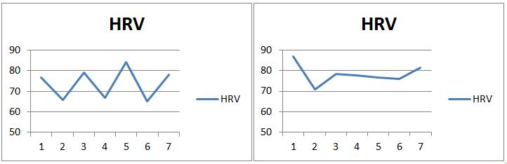
Below are two separate HRV trends I pulled from a training cycle I did last year at week 1 and week 8.

Week 1 and Week 8

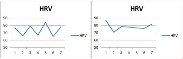
If someone were taking once per week recordings, or pre and post training phase recordings on isolated days, you can see how they can get entirely different results based on which day they measured. Suppose measures were taken on Friday’s from the above trends. These values are 84 and 76.7, respectively. However, if we look at the weekly mean values, we would get 73.6 and 78.3. From the isolated readings, one would conclude that HRV decreased nearly 10 points. However, the weekly mean shows an entirely different change (HRV actually increased from 73.6 to 78.3).  Therefore, it’s quite clear that when averaged weekly, HRV scores allow for more meaningful interpretation.

  Isolated Measure (Friday) Weekly Mean
Week 1 84 73.6
Week 8 76.7 78.3

See the following papers for more on weekly mean vs. isolated recordings (Le Meur et al. 2013; Plews et al. 2012; Plews et al. 2013)


One limitation of the weekly mean value is that is does not reflect the fluctuation in scores throughout the 7 day period. A simple way of determining this is to calculate the coefficient of variation (CV) from the 7 day HRV values (see Plews et al. 2012 for more on CV).

The coefficient of variation is calculated as follows;

CV = (Standard Deviation/Mean)x100

Below is 9 weeks worth of data from a training cycle I performed early last year that resulted in some personal records (PR’s) and was discussed in this post. This time, in addition to the weekly mean values I have also calculated the CV for each week.

9 weeks CV and Mean

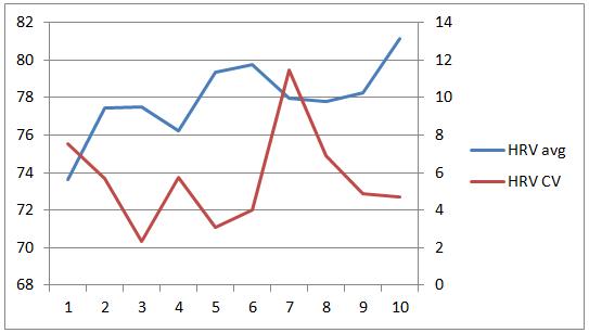
Without going into too much detail about the training cycle (see the original post for that), I will highlight a few keep observations.

HRV Avg HRV CV Brief Notes
73.6 7.5 1st week after detraining, Good
77.4 5.6  Good
77.5 2.3  Good
76.2 5.7 Stress, poor sleep, deload
79.37 3.0  Good
79.7 4.0  Good
77.9 11.4 Stressful week
77.8 6.8 ↑ intensity, ↓ Volume, Good
78.2 4.8 PR(1RMs)
81.1 4.7 Deload, Good


Below are the HRV trends from Week 1 – 4 of the cycle.

weeks 1 to 4

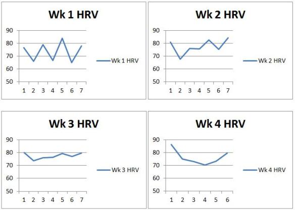
Week 1 was my first week training after about 10 days off from lifting (Christmas holidays). Clearly the trend from week 1 reflects the fatigue and recovery as I lifted on M W F that week. On week 2 I performed the same workouts on the same days but with a little more weight for each set. However, it appears (based on CV) that this may have been less stressful. In week 3, I moved to lifting 4 days/week with moderate loads and CV decreases further. Interestingly, the following week (week 4), the weights feel heavy, I feel pretty rough and I take an unplanned deload (CV increases, mean decrease).

Further analysis of the CV and weekly mean can include calculating the smallest worthwhile change (see Buchheit, 2014) to see if a change is practically meaningful. (Will do this in the future once I figure out how to display SWC on a chart).

The point of this post was to introduce the CV concept for those who may not be familiar. I believe that the CV likely provides information regarding stress, fatigue and adaptation that the weekly mean may not reflect. Therefore, the CV and mean values should be considered together.

References:

Buchheit, M. (2014). Monitoring training status with HR measures: do all roads lead to Rome? Frontiers in physiology5. http://journal.frontiersin.org/Journal/10.3389/fphys.2014.00073/full

Le Meur, Y., Pichon, A., Schaal, K., Schmitt, L., Louis, J., Gueneron, J., … & Hausswirth, C. (2013). Evidence of parasympathetic hyperactivity in functionally overreached athletes. Medicine and Science in Sports and Exercise45(11), 2061-2071.

Plews, D. J., Laursen, P. B., Kilding, A. E., & Buchheit, M. (2012). Heart rate variability in elite triathletes, is variation in variability the key to effective training? A case comparison. European journal of applied physiology112(11), 3729-3741.

Plews, D. J., Laursen, P. B., Kilding, A. E., & Buchheit, M. (2013a). Evaluating training adaptation with heart-rate measures: a methodological comparison. International Journal of Sports Physiology & Performance8(6).

HRV in a bit more detail: Part 2

Part 1 of this series provided information on heart function, ECG basics, HRV basics and how the Autonomic nervous system influences heart rate. For Part 2, I’ll discuss and display basic HRV analysis concepts to try and enhance your understanding of HRV.  I’ll relate as much of this discussion as possible to smart-phone based HRV tools as it is unlikely that most readers of this site have access to an ECG.

Athlete vs. Non-Athlete

Fit individuals generally have lower resting heart rates and greater parasympathetic activity at rest. These adaptations to training may be a result of both intrinsic heart adaptations (SA node remodeling, increase in ventricle capacity) and autonomic adaptations (greater vagal activity).

Below is an ECG segment from a collegiate male endurance athlete. This sample is likely capturing the normal fluctuation in heart rate that occurs in response to respiration (breathing). Heart rate tends to speed up on inspiration and slow down on expiration. The technical term used to describe this phenomenon is “Respiratory Sinus Arrhythmia”.

athlete ECG RSA1

Endurance Athlete ECG

For comparison, below is a screen shot of a healthy non-athlete ECG. Here, you can clearly see a higher resting heart rate and less variability.

Non-athlete ECG

Non-athlete ECG

The Excel snap shot below is what R-R interval data looks like once exported from the ECG software (Acqknowledge in this case) to a workbook. Though specialized HRV software is much more functional, it’s certainly possible to perform some time series (statistical) analysis on the R-R interval data with basic excel functions (i.e. Standard Deviation, Mean R-R Interval, RMSSD, etc.). Today, we’ll focus primarily on RMSSD as this parameter appears to be the preferred HRV index for athlete monitoring (See Plews et al. 2013 and this for more on RMSSD).

R-R Intervals

R-R Intervals

Tachogram

With HRV software analysis, ECG recordings are converted to a tachogram, which plot the successive R-R intervals on the y-axis and the number of beats within the ECG segment on the x-axis. This provides a nice visual representation of heart rate variability over a given time and makes for easy software analysis.

Below is a 5 minute ECG segment from an endurance athlete converted to a tachogram with our Nevrokard HRV software. Notice how the R-R intervals vary considerably over a broad range. The time domain values follow.

Endurance Athlete Tachogram

Endurance Athlete Tachogram

EAstats1

In contrast, below is the tachogram and time domain analysis of an age matched non-endurance athlete for comparison. Note how the R-R intervals are relatively stable and within a narrow range, demonstrating less variability.

Non-athlete Tachogram

Non-athlete Tachogram

NAstats1

To put this in perspective for the good folks using ithlete or BioForce, I’ll convert the raw RMSSD values (displayed in the “Summary Statistics” screen shots above) to ithlete/BioForce values. To do this, we simply log transform the raw RMSSD and multiply it by 20 (lnRMSSDx20). Keep in mind that the ithlete uses a 55-sec test and BioForce uses 2.5-min test. The values shown here are from 5-min ECG samples, but you get the idea.

rmssd conversion

Ectopic Beats and Artifacts

Last post, I discussed “normal” beats originating from the SA node. Any beats originating from outside the SA node disturb cardiac rhythm and can therefore impact HRV. These are called ectopic beats. Electrical interference, or excessive noise or movement can create “artifacts” which can also affect the data. It’s important to manually inspect ECG data for ectopic beats or artifacts and correct them (replace with the adjacent “normal” cycle) or discard the ECG sample entirely if there are excessive disturbances. Most smart-phone HRV tools do not provide R-R interval data and therefore manual inspection for ectopic beats is impossible. Conveniently, devices such as ithlete and BioForce are designed to automatically detect and correct irregular beats. For example, the application will detect and replace R-R intervals that are unlikely to occur in healthy, resting individuals (e.g., R-R intervals below 500ms or above 1800ms). I’d assume OmegaWave Pro, SweetBeat and other devices also have this feature.

Below is an example of an ectopic beat from an ECG which appears to be a premature atrial contraction. You’ll see this again in a moment on the tachogram as well.

ectopic1

Measurement Protocol

For athlete monitoring, HRV data is ideally collected as soon after waking in the morning as possible after bladder emptying.  We want as close to resting conditions as possible. It would be wise to avoid checking e-mails, text messages and anything else that can alter mood, excite you, upset you, etc. Even water consumption will have an acute impact on HRV. Consistency of measurement protocol and time of measurement are important for longitudinal monitoring. In addition, being as motionless as possible and undisturbed is equally as important.

In the screen shot below towards the right hand side, we can clearly see when the individual gets restless and moves or adjusts his position. We can also see the ectopic beat that occurs toward the start of the measure (same ectopic beat shown above in the ECG). Slight and subtle movements can clearly impact heart rate so be as still as possible when you perform your measures at home.

ectopic_disturbed tachogram

In the tachogram below, notice how heart rate changes considerably at around the 10 minute mark. This is a result of a researcher entering the exam room where the subject was resting during an ECG recording. Clearly, the resting condition was disturbed as the subject was excited/stressed from the person entering the room. Thus, do your best to remain as undisturbed as possible when performing a measure at home.

disturbed measure 10min

All data shown today were from supine ECG recordings. Next post I’ll discuss and show HRV changes in response to postural change (i.e., from supine to standing).

HRV in a bit more detail

Over the next several posts I will attempt to provide a little more depth to the typical explanations of heart rate variability that I’ve provided in the past. I will be displaying ECG data and HRV software screen shots to provide a better visual representation of HRV analysis. I will present and discuss things like;

  • How HRV data is often collected and analyzed
  • ECG basics
  • What respiratory sinus arrhythmia looks like
  • What an ectopic beat looks like
  • What a tachogram is and looks like (HRV software)
  • Comparing athlete to non-athlete ECG/HRV data
  • Looking at supine and standing ECG/HRV data
  • Looking at paced vs. spontaneous breathing data and how it affects HRV
  • Showing how subtle errors can impact an HRV measurement
  • Discussing HRV research questions that my colleague and I are investigating here in our lab
  • Whatever else seems  relevant as I get writing

Today’s post will serve as a brief, but slightly more in depth introduction to heart rate physiology. To really get a handle on HRV, it’s important to have an understanding of the interplay between the brain and heart and the details therein. I encourage interested readers to check out an actual physiology text for a more elaborate and detailed discussion for which I’ll provide a few recommendations at the end.

Heart Rate

The human heart is equipped with an intrinsic pacemaker within the wall of the right atrium called the sinoatrial node (SA node).  The SA node randomly depolarizes, generating action potentials that ultimately result in a contraction (heart beat). All heart beats that originate from the SA node are “normal” beats and provide normal cardiac rhythm. However, as we’ll get into eventually when I display some ectopic beats, depolarization also regularly occurs in other areas within the myocardium, which if reach threshold, can initiate a contraction on its own. Non SA node action potentials disturb cardiac rhythm that is ideally dictated by the SA node (more on ectopic beats in future). Left alone, the SA node would give you a resting heart rate of about 100 beats per minute. Obviously, healthy individuals have much lower heart rates while at rest. Other times, we can experience quite high elevations in heart rate to facilitate blood distribution requirements (e.g., during physical activity). We’ll get into how these changes in heart rate occur momentarily.

In the lab, we can evaluate heart beat information with electrocardiographic (ECG) recordings. An ECG detects electrical currents at the surface of the skin generated by the action potentials that propagate through the heart. In our lab, since we’re mainly interested in heart rate variability and not intricate ECG analysis, we use a simple, modified lead II electrode placement. From the ECG we can observe 3 distinct patters that represent the electrical conductivity involved in the cardiac cycle;

pqrst

P wave – Displays as a small upward deflection and represents atrial depolarization. The P wave indicates that the impulse originated from the SA node and therefore results in a “normal” beat.

QRS Complex – Begins with a shallow downward deflection (Q), followed by a tall upward deflection (R) and ends with another downward deflection (S). Collectively, this represents ventricular depolarization.

T wave – Oftend described as dome-shaped in appearance and represents ventricular repolarization

As you can see, the R wave has a high peak making measurements between cardiac cycles rather easy. The elapsed time between two R waves creates an R-R interval. The time between R-R intervals varies across successive R-R intervals and is termed heart rate variability. In the screen shot below of the AcqKnowledge software, notice how the space between R waves (the tall peaks) is inconsistent as some intervals are wider and some are more narrow.

ECG


Centrally Mediated Cardiac Control

Now we’ll return to our discussion on heart rate control. Heart rate is influenced by both intrinsic and extrinsic mechanisms, however for this discussion, our interest is primarily with central nervous system regulation of cardiac control via autonomic innervations of the heart. Heart rate is largely mediated by both sympathetic and parasympathetic influence which originates in the cardiovascular center of the brain. The cardiovascular center is located on the lower portion of the brain stem at the medulla oblongata. From here, sympathetic neurons extend from the brain, through the spinal cord and directly into the heart. Increased sympathetic activity increases the release of norepinephrine which speeds up SA node depolarization (increases heart rate) and increases the force of contraction. This response occurs to facilitate increased blood distribution requirements that may arise due to physical activity, stress, standing up, etc.

Parasympathetic influence of the heart occurs via the Vagus nerve (10th cranial nerve) which originates in the medulla and has axons that terminate directly into the heart. Vagal stimulation elicits an inhibitory effect on the SA node via release of acetylcholine, effectively reducing heart rate and is associated with “rest and digest” activity. Since vagal activity inhibits SA node activity, vagal withdrawal will result in less SA node inhibition and allow the heart to beat faster. At the onset of exercise, the initial increase in heart rate is a result of vagal withdrawal with a progressive increase in sympathetic activity as exercise persists (Yamamoto et al. 1991).

Since heart rate is directly affected by autonomic activity, it serves as a relatively simple marker for us to monitor to assess autonomic status. Increased parasympathetic activity will reduce heart rate and result in greater variability between R waves. In contrast, a higher heart rate with less variability (think more metronomic) is the result of reduced parasympathetic activity and possibly increased sympathetic activity.  HRV has thus become a valuable metric to monitor in athletes as it provides information regarding the relative balance of “stress” in the individual. Though I’m a proponent of HRV monitoring in athletes, its interpretation requires caution as nothing is black and white when it comes to determining an athlete’s training status from HRV, particularly from isolated measurements. Rather, taken with performance trends, psychometrics (perception of mood, soreness, fatigue, etc.), and training load, HRV becomes more meaningful.

In the next post, I will start to get into HRV analysis with some software screenshots to provide a good visual representation of HRV.


References/Recommended Reading:

Smith, D. & Fernhall, B. (2010) Advanced Cardiovascular Exercise Physiology. Human Kinetics. http://www.amazon.com/Advanced-Cardiovascular-Exercise-Physiology/dp/0736073922

Tortora, G. & Derrickson, B. (2006) Principles of Anatomy and Physiology 11th Edition. Biological Sciences Textbooks Inc.

Yamamoto, Y., Hughson, R. L., & Peterson, J. C. (1991). Autonomic control of heart rate during exercise studied by heart rate variability spectral analysis. Journal of Applied Physiology71(3), 1136-1142.

HRV Data from a High School Sprinter

Here is some more data and analysis from a nationally ranked high school sprinter (Junior) that I have using ithlete. Please note that the sprinter trains primarily with his sprint coach. I work with him roughly 3 days/week on mobility, restoration, etc.  He was an ideal candidate for monitoring HRV as he is an extremely motivated and dedicated athlete and there was no doubt in my mind that he could handle the daily measurements. The data stops in early January because he somehow broke the HRV receiver I gave him. A new one has been ordered recently I’ve been told. This data collection is primarily for observational purposes since I do not control or manipulate his training as mentioned above.

November

ZWNovTable

ZWNovtrend

  •  After 1 week of using ithlete, I had him start using the comments section and sleep score.
  • His resting heart rate was higher than I expected. I had him perform his measurements standing but in hindsight I should’ve had him do them seated based on his RHR.
  • HRV average is mid 70’s which is what I expect from an anaerobic athlete. Still would expect his HR to be at least in the high 60’s in standing position.
  • Clearly he stays up super late on weekends and sleeps in late. Been on his case about this. 

First Half of December

ZWDec1Table

 ZWDec1Trend1

  • HR/HRV average remains consistent. Coping with training well.
  • Race day on 12/7, hit a PB in his part of the relay. Not a hard race, treated as practice.
  • Reports of back soreness that persisted long enough for him to seek treatment (documented in next table).

Christmas Break – Second Half of December & Early January 

ZWXmasTable

ZWXmasTrend

  •  This last section of data is from his Christmas break. Interestingly his HRV average drops and his RHR increases. I attribute this to the change in routine (off of school), staying up late regularly, etc. I also notice changes in my HRV when my routine is interrupted. The body likes consistency.
  • Things appear to be going well though as he seldom gets below baseline scores (amber).
  • Race day on 1/6 and hits a PB on 60m.

Given that this athlete is still young and taking advantage of “newbie” strength gains, I would expect him to hit PB’s relatively consistently on the track. Based on his trend, fatigue was never really an issue. More training may have been well tolerated.

I’d like to get him to start using the training load feature too now to get a better idea of how hard his workouts are (perceptively).