There is very little longitudinal HRV data within the research, particularly in team sport athletes. In many cases, HRV will be assessed pre and post or pre, mid and post of a pre-season camp or what have you. This is very likely due to the inconvenience of acquiring this type of data in athletic populations. For the study to be research quality, validated tools must be used (ECG, Polar, Suunto, Omegawave, etc.). In addition, standard measurement procedures are required to ensure that the data is of sufficient quality. This generally involves a 5 minute rest period followed by a 5 minute recording. However, some researchers have used shorter resting and recording durations. Measurement standards for athlete monitoring in the field need to be developed. This is an area my colleague Dr. Esco and I are working on in our lab. This includes cross-validating field HRV tools, assessing the suitability of shorter recording durations and determining the time course for stabilization of HRV (i.e., how long should the resting condition be prior to recording).
Apart from the issue of valid and reliable tools and measurement protocols, another major issue that prevents HRV from being widely used as a component of a comprehensive athlete monitoring program is compliance. Due to day to day variations it is highly unlikely that a single HRV recording per week is sufficient. A recent paper by Le Meur et al. (2013) found that:
“using mean weekly values obtained from daily HRV recordings, rather than isolated HRV assessments, may improve the diagnostic utility of HRV indices in endurance-trained athletes to assess training-induced adaptations of the autonomic nervous system. The present results suggest that the day-to-day variability of HRV values is too high to allow clear detection of autonomic modulations associated with F-OR using single-day values.”
Understanding that daily HRV recordings can be difficult to obtain from our athletes, Plews et al. (2013) sought to determine what the minimum measurement frequency is that still appropriately reflects the weekly mean value.
“We have previously demonstrated HRV values averaged over 1 week provide a superior representation of training-induced changes than HRV values taken on a single day. In the current study, we have shown that HRV values averaged at random over a minimum number of 3 days will allow for an equivalent representation of training adaptation than values averaged for up to 7 days in trained triathletes. Conversely, recreational athletes will need a slightly greater number of days averaging (~5 days) due to their greater day-to-day variations in Ln rMSSD values.”
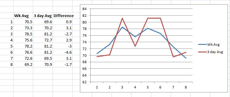
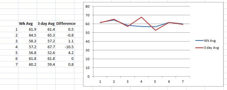
Last March, I posted some data that assessed the trends of daily vs. once per week and twice per week HRV recordings here. Today I’d like to revisit this topic. However, in this post I will be comparing weekly mean values to 3 day/week values. In the study mentioned above by Plews et al., the 3 days were randomly selected and were compared with performance changes. I’ve elected to consistently use Mon-Wed-Fri recordings to assess how a more structured and consistent approach would work and compare to the weekly mean trend. Working with a team of athletes, it would be much easier to designate 3 specific week days as HRV recording days. However, which 3 days are selected should likely depend on the training/competition schedule. Selecting days that all fall after intense training/competition may skew the results and not sufficiently reflect the recovery seen on days after lower intensity or rest days.
Below is the first week of every month from the last year (Jan 2013 – Jan2014) of my ithlete data. I figured 1 week per month would sufficiently show trend changes due to changes in fitness, lifestyle etc, without having to spending too much time analyzing data in excel for every week of the year.

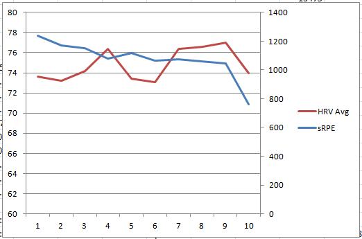
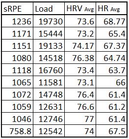
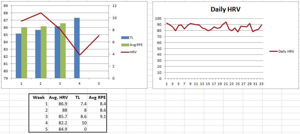
Below is HRV data from a Collegiate Cross Country athlete throughout the fall competitive season.
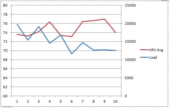
Below is some in-season data from a female Collegiate soccer player.
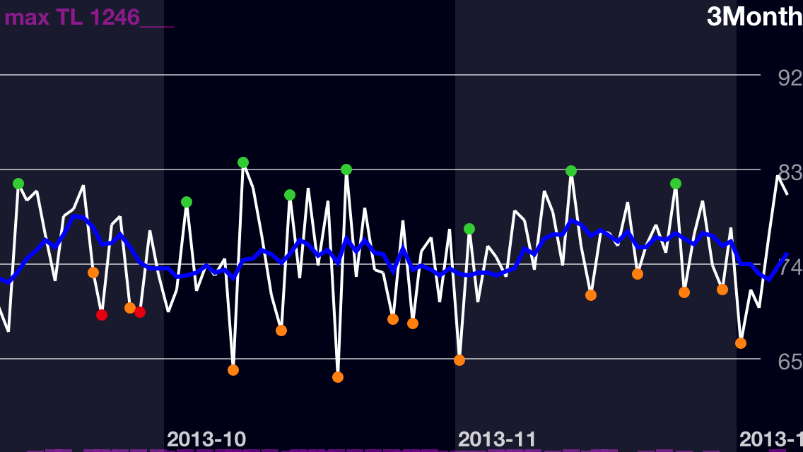
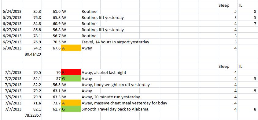
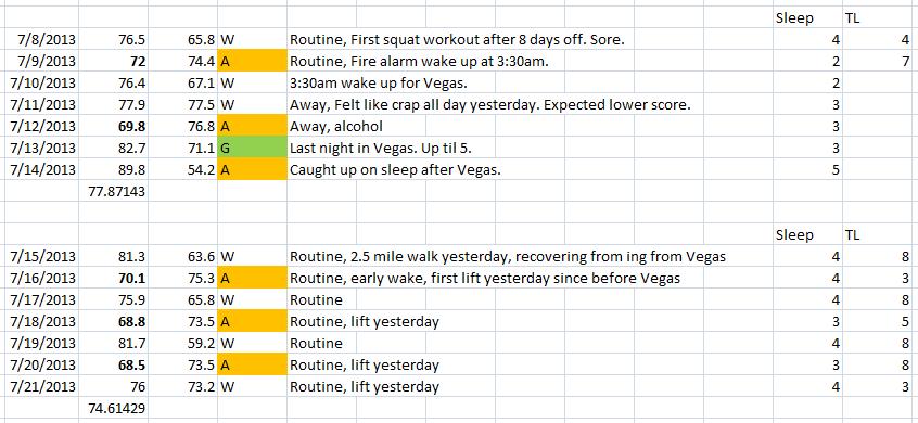
Lastly, below I’ve posted a randomly selected week from each month over 9 months from a competitive male powerlifter with Cerebral Palsy.

It was specifically stated that non-elite athletes may require more than a 3 day average to sufficiently reflect performance changes. This is due to a higher degree of variation in day to day measures.
“Conversely, recreational athletes will need a slightly greater number of days averaging (~5 days) due to their greater day-to-day variations in Ln rMSSD values.” Plews et al.
None of the above athletes are “elite” (as much as I’d like to think I am). Clearly there are a few weeks that do not match up for each data set, but the 3 day average (drawn from Mon-Wed-Fri in each set) appears to follow the weekly mean trend reasonably well. Having your athletes record HRV on a mobile device 3 days per week would certainly be more manageable than daily recordings. I intend to investigate this more officially in the future.
Refs:
Le Meur, Y., Pichon, A., Schaal, K., Schmitt, L., Louis, J., Gueneron, J., … & Hausswirth, C. (2013). Evidence of Parasympathetic Hyperactivity in Functionally Overreached Athletes. Medicine and Science in Sports and Exercise.
Plews, D. J., Laursen, P. B., Le Meur, Y., Hausswirth, C., Kilding, A. E., & Buchheit, M. (2013). Monitoring Training With Heart Rate Variability: How Much Compliance is Needed for Valid Assessment?. International Journal of Sports Physiology and Performance. Ahead of print.